Tag: GitHub

  • Digging into the British Empire with R: Lexical topics, part 5

    Some of the most powerful (and interesting) features of working with R on corpus analysis involve exploring technical features of texts. In this script, I use a some well-known R packages for text analysis like tidyr and tidytext, combined with ggplot2, which I used in the previous post, to analyze and visualize textual data.

    This comnbination allows us to do things like find word frequences in particular subsets of the corpus. In this case, I’ve selected for Rudyard Kipling and charted the 10 words he uses most frequently in the corpus:

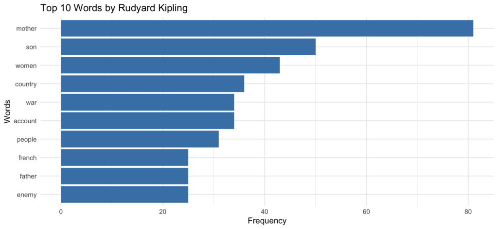
    To accomplish this, I filtered for texts by Kipling, unnested the tokens, generated a word count, and plotted the words in a bar graph. Here’s the code:

    # Filter for a specific author in the corpus and tokenize text into words. Here
    # I've used Kipling 
    word_freq <- empire_texts %>%
      filter(author == "Kipling, Rudyard") %>%
      unnest_tokens(word, text) %>%
      # Remove stop words and non-alphabetic characters
      anti_join(stop_words, by = "word") %>%
      filter(str_detect(word, "^[a-z]+$")) %>%
      # Count word frequencies
      count(word, sort = TRUE) %>%
      top_n(10, n)
    
    # Create bar graph
    ggplot(word_freq, aes(x = reorder(word, n), y = n)) +
      geom_bar(stat = "identity", fill = "steelblue") +
      coord_flip() +
      labs(title = "Top 10 Words by Rudyard Kipling",
           x = "Words", y = "Frequency") +
      theme_minimal()

    I also selected the top 10 bigrams and filtered for author, in this case H. Rider Haggard:

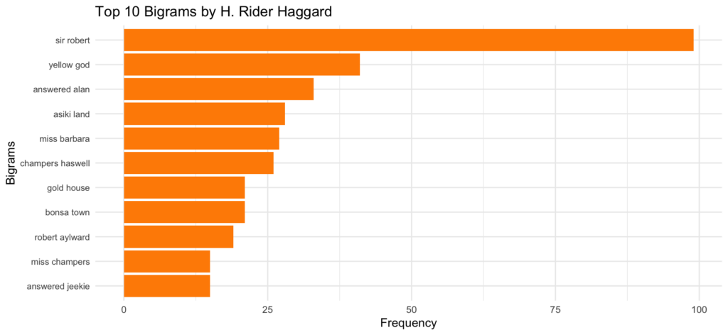
    In this case, I was just interested in seeing any bigrams, but depending on your analysis, you might want to see, for example, what the first word in a bigram is if the second word is always “land.” You could do that by slightly modifying the script and including a line to filter word2 as land. For example:

    bigram_freq <- empire_texts %>%
      filter(author == "Haggard, H. Rider (Henry Rider)") %>%
      unnest_tokens(bigram, text, token = "ngrams", n = 2) %>%
      filter(!is.na(bigram)) %>%
      separate(bigram, into = c("word1", "word2"), sep = " ") %>%
      # Filter for bigrams where word2 is "land"
      filter(word2 == "land") %>%
      filter(!word1 %in% stop_words$word) %>%
      unite(bigram, word1, word2, sep = " ") %>%
      count(bigram, sort = TRUE) %>%
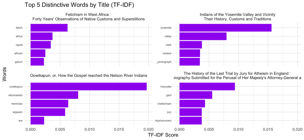
      top_n(10, n)

    Finally, I’ve used TF-IDF (Term Frequency-Inverse Document Frequency) to chart the top 5 most distinctive words by title. The titles are randomly generated from the corpus with set seed (which I’ve set to 279 in my script), but you could regenerate with random titles by changing the set seed number.

    Here’s the script for that:

    # Filter, tokenize, and calculate TF-IDF
    tfidf_data <- empire_texts %>%
      filter(title %in% sample_titles) %>%
      unnest_tokens(word, text) %>%
      anti_join(stop_words, by = "word") %>%
      count(title, word, name = "n") %>%
      bind_tf_idf(word, title, n) %>%
      # Get top 5 words per title by TF-IDF
      group_by(title) %>%
      slice_max(order_by = tf_idf, n = 5, with_ties = FALSE) %>%
      ungroup()
    
    # Create faceted bar plot
    ggplot(tfidf_data, aes(x = reorder_within(word, tf_idf, title), y = tf_idf)) +
      geom_bar(stat = "identity", fill = "purple") +
      facet_wrap(~title, scales = "free_y") +
      coord_flip() +
      scale_x_reordered() +
      labs(title = "Top 5 Distinctive Words by Title (TF-IDF)",
           x = "Words", y = "TF-IDF Score") +
      theme_minimal() +
      theme(axis.text.y = element_text(size = 6))

    Needless to say, you could run this with as many titles as you chose, though the graph gets a little wonky if you run too many–and the process can slow down considerably depending on the size of the corpus.

    It’s worth noting that these plots can be written to an R document called Quarto and published on the web (with a free account) via RPubs. This can help if want to use charts for a presentation, or even if you just want the chart to display online in a more versatile environment. Maybe I’ll write a series on creating presentations in RStudio at some point.

    Here’s the third and final script for our British Empire sentiment analysis.

    Stay tuned for the next project.

  • Digging into the British Empire with R: Loading a corpus, part 3

    Alright, here’s the R script I used to generate the corpus. As you can see, there are a lot of ways this could be tweaked. I didn’t do this, but it would be possible (and probably even preferable) to run the search, collect the data, and manually sift through the results if you have a relatively small corpus.

    # Install packages  
    install.packages("gutenbergr")
    install.packages("dplyr")
    install.packages("stringr")
    
    # Load required libraries
    library(gutenbergr)
    library(dplyr)
    library(stringr)
    
    # Get the Gutenberg metadata
    gb_metadata <- gutenberg_works()
    
    # Define search terms related to British Empire
    search_terms <- c("india", "colony", "colonial", "empire", "africa", "asia", 
                      "imperial", "natives", "british", "england", "victoria", 
                      "trade", "east india", "conquest")
    
    # First approach: Find works with publication dates in the 19th century where possible
    # Many Gutenberg works have no publication dates
    dated_works <- gb_metadata %>%
      filter(
        language == "en",
        !is.na(gutenberg_author_id),
        !str_detect(title, "Bible|Dictionary|Encyclopedia|Manual|Cookbook")
      ) %>%
      # But some do, so let's make sure we get those 
      filter(
        !is.na(gutenberg_bookshelf),
        str_detect(gutenberg_bookshelf, "1800|19th")
      )
    
    # Second approach: Find popular authors from the 19th century
    empire_authors <- c("Rudyard Kipling", "Joseph Conrad", "Charles Dickens", 
                        "H. Rider Haggard", "Robert Louis Stevenson", "Anthony Trollope", 
                        "E.M. Forster", "John Stuart Mill", "Thomas Macaulay", 
                        "Thomas Babington Macaulay", "James Mill", "George Curzon",
                        "Frederick Lugard", "Richard Burton", "David Livingstone",
                        "Henry Morton Stanley", "Mary Kingsley", "Flora Annie Steel")
    
    author_works <- gb_metadata %>%
      filter(
        language == "en",
        str_detect(author, paste(empire_authors, collapse = "|"))
      )
    
    # Third approach: Keyword search in titles
    keyword_works <- gb_metadata %>%
      filter(
        language == "en",
        str_detect(tolower(title), paste(search_terms, collapse = "|"))
      )
    
    # Combine all of the above approaches into one dataset
    empire_works <- bind_rows(dated_works, author_works, keyword_works) %>% 
      distinct() %>%
      # Use author birth/death dates to try and estimate 19th century works
      left_join(gutenberg_authors, by = "gutenberg_author_id") %>%
      filter(
        # Authors who lived during the 19th century (possibly born earlier)
        (is.na(birthdate) | 
           birthdate <= 1880) & # Born before or during most of the 19th century
          (is.na(deathdate) | 
             deathdate >= 1800)   # Died after the 19th century began
      )
    
    # View how many books we found
    print(paste("Found", nrow(empire_works), "potentially relevant works"))
    
    # Preview the first few works
    head(empire_works %>% select(gutenberg_id, title, author.x), 20)
    
    # If we have more than 1000 works, we can limit to the most relevant
    # I'm going to cap this at 1000 works, but feel freee to use a lower number if you prefer
    if(nrow(empire_works) > 1000) {
      # Calculate a relevance score based on how many search terms appear in the title
      empire_works <- empire_works %>%
        mutate(
          relevance_score = sapply(title, function(t) {
            sum(sapply(search_terms, function(term) {
              if(str_detect(tolower(t), term)) 1 else 0
            }))
          })
        ) %>%
        arrange(desc(relevance_score)) %>%
        head(1000)
    }
    
    # Download the corpus (this will take time)
    # Uncomment the two lines below when ready to download
    empire_texts <- gutenberg_download(empire_works$gutenberg_id, 
                                     meta_fields = c("title", "author"))
    
    # Take a quick look at the dataset to get a sense of how it's organized  
    View(empire_texts) 
    
    # You might want to save the metadata for future reference. If so, uncomment
    # the following lines 
    
    #write.csv(empire_works %>% select(gutenberg_id, title, author.x), 
    #          "outputs/empire_corpus_metadata.csv", row.names = FALSE)